2. CAUSAL INFERENCE IN EPIDEMIOLOGY
by Kenneth J. Rothman
In The Magic Years, Selma Fraiberg [1959] characterizes every toddler as a scientist, busily fulfilling an earnest mission to develop a logical structure for the strange objects and events that make up the world that he or she inhabits. None of us is born with any concept of causal connections. As a youngster, each person develops an inventory of causal explanations that brings meaning to the events that are perceived and ultimately leads to increasing power to control those events. Parents can attest to the delight that children take in forming causal hypotheses and then meticulously testing them, often through exasperating repetitions that are motivated mainly by the joy of scientific confirmation. At a certain age, a child will, upon entering a new room, search for a wall switch to operate the electric lighting, and upon finding one that does, repeatedly switch it on and off merely to confirm the discovery beyond any reasonable doubt. Experiments such as those designed to test the effect of gravity on free-falling liquids are usually conducted with careful attention, varying the initial conditions in subtle ways and reducing extraneous influences whenever possible by conducting the experiments safely removed from parental interference. The fruit of these scientific labors is the essential system of causal beliefs that enables each of us to navigate our complex world.
Although the method of proposing and testing causal theories is mastered intuitively by every youngster, the inferential process involved has been the subject of philosophic debate throughout the history of scientific philosophy. It is worthwhile to consider briefly the history of ideas describing the inductive process that characterizes causal inference, to understand better the modern view and its implications for epidemiology.
PHILOSOPHY OF SCIENTIFIC INFERENCE
The dominant scientific philosophy from the birth of historic scientific inquiry until the beginning of the scientific revolution was the doctrine of rationalism. According to this doctrine, scientific knowledge accumulated through reason and intuition rather than by empirical observation. In ancient Greece, the only prominent empirical science was astronomy. Nevertheless, even the observation of the heavens was belittled by Plato, who considered celestial observations an unreliable source of knowledge compared with reason [Reichenbach, 1951]. The highest form of knowledge was considered to be mathematics, a system of knowledge built upon a framework of axioms by deductive logic. The geometry of Euclid exemplifies the rationalist ideal.
Skeptics of rationalism who believed that perceptions of natural phenomena are the source and ultimate judge of knowledge developed a competing doctrine known as empiricism. The great pioneers of modern empiricism were Francis Bacon, John Locke, and David Hume. Bacon saw that earlier empiricists, though they exalted empirical science, overemphasized observation to the extent that logic played little role in the accumulation of knowledge. Bacon likened the rationalists to spiders, spinning cobwebs out of their own substance, and the older empiricists to ants, collecting material without being able to find an order in it. He envisioned a new empiricist that he likened to a bee, collecting material, digesting it, and adding to it from its own substance, thus creating a product of higher quality. According to Bacon, reason introduces abstract relations of order to observational knowledge. Bacon is famous for saying "knowledge is power," by which he meant that abstract relations imply prediction. Thus, "fire is hot" is not merely descriptive of fire but also predictive of the nature of fires not yet observed. Prediction is obtainable by a process known as inductive inference or inductive logic. Unlike deductive logic, inductive logic is not self-contained and therefore is open to error. On the other hand, deductive logic, being self-contained, cannot alone establish a theory of prediction, since it has no connection to the natural world.
Bacon formalized the process of inductive inference, demonstrating how deductive logic could never be predictive without the fruits of inductive inference. John Locke popularized the inductive methods that Bacon formalized and helped establish empiricism as the prevailing doctrine of scientific philosophy. Hume was the critic: He pointed out that inductive inference does not carry a "logical necessity," by which he meant that induction did not carry the logical force of a deductive argument. He also demonstrated that it is a circular argument to claim that inductive logic is a valid process even without a logical necessity simply because it seems to work well: No amount of experience with inductive logic could be used to justify logically its validity. Hume thus made it clear that inductive logic cannot establish a fundamental connection between cause and effect. No number of repetitions of a particular sequence of events, such as turning a light on by pushing a switch, can establish a causal connection between the action of the switch and the turning on of the light. No matter how many times the light comes on after the switch has been pressed, the possibility of coincidental occurrence cannot be ruled out. This incompleteness in inductive logic became known as "Hume's problem."
Various philosophers have tried to provide answers to Hume's problem. The school of logical positivism that emerged from the Vienna Circle of philosophers incorporated the symbolic logic of Russell and Whitehead's Principia Mathematica into its analysis of the verification of scientific propositions. The tenet of this philosophy was that the meaningfulness of a proposition hinged on the empirical verifiability of the proposition according to logical principles. This view was inadequate as a philosophy of science, however, because, as Hume had indicated, no amount of empirical evidence can verify conclusively the type of universal proposition that is a scientific law [Popper, 1965]. Hume's problem remained unanswered by this approach.
Confronting the hopelessness of conclusive verification, some philosophers of science adopted a graduated system of verifiability, embodied by
the logic of probabilities proposed by Rudolph Carnap. Under this philosophy, scientific propositions are evaluated on a probability scale. Upon empirical testing, hypotheses become more or less probable depending on the outcome of the test. The description by Heisenberg of the "uncertainty principle" and the acceptance of quantum mechanics by physicists early in the twentieth century fostered this probabilistic view of scientific confirmation. Philosophers, influenced strongly by contemporary physicists, abandoned the search for causality:The picture of scientific method drafted by modern philosophy is very different from traditional conceptions. Gone is the ideal of the scientist who knows the absolute truth. The happenings of nature are like rolling dice rather than like revolving stars; they are controlled by probability laws, not by causality, and the scientist resembles a gambler more than a prophet [Reichenbach, 1951].
The notion of verifiability by probabilistic logic did not take root. The inadequacy of this philosophy was revealed by Karl Popper, who demonstrated that statements of probabilistic confirmation, being neither axioms nor observations, are themselves scientific statements requiring probability judgments [Popper, 1965]. The resulting "infinite regress" did not resolve Hume's criticism of the inductive process.
Popper proposed a more persuasive solution to Hume's problem. Popper accepted Hume's point that induction based on confirmation of a cause-effect relation, or confirmation of a hypothesis, never occurs. Furthermore, he asserted that knowledge accumulates only by falsification. According to this view, hypotheses about the empirical world are never proved by inductive logic (in fact, empirical hypotheses can never be "proved" at all in the sense that something is proved in deductive logic or in mathematics), but they can be disproved, that is, falsified. The testing of hypotheses occurs by attempting to falsify them. The strategy involves forming the hypothesis by intuition and conjecture, using deductive logic to infer predictions from the hypothesis, and comparing observations with the deduced predictions. Hypotheses that have been tested and not falsified are confirmed only in the sense that they remain reasonably good explanations of natural phenomena until they are falsified and replaced by other hypotheses that better explain the observations. The empirical content of a hypothesis, according to Popper, is measured by how falsifiable the hypothesis is. The hypothesis "God is one" has no empirical content because it cannot be falsified by any observations. Hypotheses that make many prohibitions about what can happen are more falsifiable and therefore have more empirical content, whereas hypotheses that make few prohibitions have little empirical content. Lack of empirical content, however, is not equivalent to lack of validity: A statement without empirical content relates to a realm outside of empirical science.
Popper also rejected the abandonment of causality. He argued forcefully
that an indeterminist philosophy of science could have only negative consequences for the growth of knowledge, and that Heisenberg's "uncertainty principle" did not place strict limits on scientific discovery. For Popper, belief in causality was compatible with uncertainty, since scientific propositions are not proved: They are only tentative explanations, to be replaced eventually by better ones when observations falsify them. It is worth noting that at least one prominent physicist, like Popper, did not relinquish a belief in causality:... I should not want to be forced into abandoning strict causality without defending it more strongly than I have so far. I find the idea quite intolerable that an electron exposed to radiation should choose of its own free will, not only its moment to jump off, but also its direction. In that case, I would rather be a cobbler, or even an employee in a gaming house, than a physicist [Einstein, 1924].
Recent developments in theoretical physics seem to promise vindication of Einstein's faith in causality [Waldrop, 1985].
Popper's philosophy of science has many adherents, but recent scientific philosophers temper the strict falsificationism that he proposed. Brown [1977] cites three fundamental objections to the Popperian view: (1) refutation is not a certain process, since it depends on observations, which can be erroneous; (2) deduction may provide predictions from hypotheses, but no logical structure exists by which to compare predictions with observations; and (3) the infrastructure of the scientific laws in which new hypotheses are imbedded is itself falsifiable, so that the process of refutation amounts only to a choice between refuting the hypothesis or refuting the infrastructure from which the predictions emerge. The last point is the essential view of the post-Popperian philosophers, who argue that the acceptance or rejection of a scientific hypothesis comes through consensus of the scientific community [Brown, 1977] and that the prevailing scientific viewpoint, which Kuhn [1962] has referred to as "normal science," occasionally undergoes major shifts that amount to scientific revolutions. These revolutions signal a decision of the scientific community to discard the infrastructure rather than to falsify a new hypothesis that cannot be easily grafted onto it.
A GENERAL MODEL OF CAUSATION
Philosophers of science have clarified the understanding of the process of causal inference, but there remains the need, at least in epidemiology, to formulate a general and coherent model of causation to facilitate the conceptualization of epidemiologic problems. Without such a model, epidemiologic concepts such as causal interactions, induction time, and the proportion of disease attributable to specific causes would have no ontologic foundation.
We can define a cause of a disease as an event, condition, or characteristic that plays an essential role in producing an occurrence of the disease. Causality is a relative concept that can be understood only in relation to conceivable alternatives. Smoking one pack of cigarettes daily for 10 years may be thought of as a cause of lung cancer, since that amount of smoking may play an essential role in the occurrence of some cases of lung cancer. But this construction postulates some lesser degree of smoking, such as nonsmoking, as the alternative. Smoking only one pack of cigarettes daily for 10 years is a preventive of lung cancer if the alternative is to smoke 2 packs daily for the same period, because some cases of lung cancer that would have occurred from smoking 2 packs daily will not occur. Analogously, we cannot consider that taking oral contraceptives is a cause of death (by causing fatal cardiovascular disease) unless we know what the alternative is; if the alternative is childbirth, a life-threatening event, taking oral contraceptives may prevent death. Thus, causation and prevention are relative terms that should be viewed as two sides of the same coin.
Concept of Sufficient Cause and Component Causes
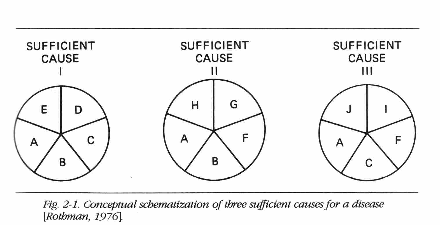
Concepts of cause and effect are established early in life. The child who repeatedly drops a toy and watches it fall or tips a glass and observes the milk spilling is applying his own method of reasoning to causal propositions and in so doing is working out his own concept of causation. A characteristic of such early concepts is the assumption of a one-to-one correspondence between the observed cause and effect in the sense that each such cause is seen as necessary and sufficient in itself to produce the effect. Thus, the flick of a light switch makes the lights go on. The unseen causes that also operate to produce the effect are unappreciated: the need for an unspent bulb in the light fixture, wiring from the switch to the bulb, and voltage to produce a current when the circuit is closed. To achieve the effect of turning on the light, each of these is equally as important as moving the switch because absence of any of these components of the causal constellation will prevent the effect. For many people, the roots of early causal thinking persist and become manifest in attempts to find single causes as explanations for observed phenomena. But experience and reflection should easily persuade us that the cause of any effect must consist of a constellation of components that act in concert [Mill, 1862]. A "sufficient cause" may be defined as a set of minimal conditions and events that inevitably produce disease; "minimal" implies that none of the conditions or events is superfluous. In disease etiology, the completion of a sufficient cause may be considered equivalent to the onset of disease. For biologic effects, most and sometimes all of the components of a sufficient cause are unknown [Rothman, 1976].
For example, smoking is a cause of lung cancer, but by itself it is not a sufficient cause. First, the term smoking is too imprecise to be used in a causal description. One must specify the type of smoke, whether it is filtered or unfiltered, the manner and frequency of inhalation, and the duration of smoking. More important, smoking, even defined explicitly, will not cause cancer in everyone. So who are those who are "susceptible" to the effects of smoking, or, to put it in other terms, what are the other components of the causal constellation that act with smoking to produce lung cancer? When causal components remain unknown, there is an inclination to assign an equal risk to all individuals whose causal status for some components is known and identical. Thus, heavy cigarette smokers are said to have approximately a 10 percent lifetime risk of developing lung cancer. There is a tendency to think that all of us are subject to a 10 percent probability of lung cancer if we were to become heavy smokers, as if the outcome, aside from smoking, were purely a matter of chance. It is more constructive, however, to view the assignment of equal risks as reflecting nothing more than our ignorance about the determinants of lung cancer that interact with cigarette smoke. It is likely that some of us could engage in chain smoking for many decades without the slightest possibility of developing lung cancer. Others are or will become "primed" by presently unknown circumstances and need only to add cigarette smoke to the nearly sufficient constellation of causes to initiate lung cancer. In our ignorance of these hidden causal components, the best we can do in assessing risk is to assign the average value to everyone exposed to a given pattern of known causal risk indicators. As knowledge expands, the risk estimates assigned to people will approach one of the extreme values, zero or unity.
Each constellation of component causes represented in Figure 2-1 is minimally sufficient (i.e., there are no redundant or extraneous component causes) to produce the disease. Component causes may play a role in one, two or all three causal mechanisms.
Strength of Causes
Figure 2-1 does not depict aspects of the causal process such as sequence of action, dose, and other complexities. These aspects of the causal process can be accommodated by the model by an appropriate definition of each causal component. The model and diagram do facilitate an understanding of some important epidemiologic concepts. Imagine, for example, that in Sufficient Cause I, A, B, C, and D all are factors commonly present or experienced by people. Suppose E were rare. Although all factors are causes, E would appear to be a stronger determinant of disease because those with E differ greatly in risk from those without E. The other, more common component causes result in smaller differences in risk between those with and those without the causes because the rarity of E keeps the risks from all the other factors low. Thus, the apparent strength of a cause is determined by the relative prevalence of component causes. A rare factor becomes a strong cause if its complementary causes are common. It should
be apparent that, although it may have tremendous public health significance, the strength of a cause has little biologic significance in that the same causal mechanism is compatible with any of the component causes being strong or weak. The identity of the constituent components of the cause is the biology of causation, whereas the strength of a cause is a relative phenomenon that depends on the time- and place-specific distribution of component causes in a population.Interaction Among Causes
Two component causes in a single sufficient cause are considered to have a mutual biologic interaction. The degree of observable interaction depends on the actual mechanisms responsible for disease. For example, in Figure 2-1, if G were a hypothetical substance that had not been created, no disease would occur from Sufficient Cause II; as a consequence, factors B and F are biologically independent. Now suppose that the prevalence of C is reduced because it is replaced by G or something that produced G. In this case the disease that occurs comes from Sufficient Cause II rather than from I or III, and as a consequence, B and F interact biologically. Thus, the extent of biologic interaction between two factors is in principle dependent on the relative prevalence of other factors.
Proportion of Disease Due to Specific Causes
In Figure 2-1, assuming that the three sufficient causes are the only ones operating, what proportion of disease is caused by A? The answer is all of it; without A, there is no disease. A is considered a "necessary cause." What proportion is due to B? B causes disease through two mechanisms, I and II, and all disease arising through either of these two mechanisms is due to B. This is not to say, of course, that all disease is due to A alone, or that a proportion of disease is due to B alone; no component cause acts alone.
It is understood that these factors interact with others in producing disease.
Recently it was proposed that as much as 40 percent of cancer is caused by occupational exposures. Many scientists argued against this claim [Higginson, 1980; Ephron, 1984]. One of the arguments used in rebuttal was as follows: x percent of cancer is caused by smoking, y percent by diet, z percent by alcohol, and so on; when all these percentages are added up, only a few percent are left for occupational causes. This argument is based on a naive view of cause and effect, which neglects interactions. There is, in fact, no upper limit to the sum that was being constructed; the total of the proportion of disease attributable to various causes is not 100 percent but infinity. Similarly, much publicity attended the pronouncement that 90 percent of cancer is environmentally caused [Higginson, I960]; by extension of the previous argument, however, it is easy to show that 100 percent of any disease is environmentally caused, and 100 percent is inherited as well. Any other view is based on a naive understanding of causation.
Induction Period
The diagram of causes also gives us a model for conceptualizing the induction period, which may be defined as the period of time from causal action until disease initiation. If, in Sufficient Cause I, the sequence of action of the causes is A, B, C, D, and E, and we are studying the effect of B, which, let us assume, acts at a point in time, we do not observe the occurrence of disease immediately after B acts. Disease occurs only after the sequence is completed, so there will be a delay while C, D, and finally E act. When E acts, disease occurs. The interval between the action of B and the disease occurrence is the induction time for the effect of B. A clear example of a lengthy induction time is the cause-effect relation between exposure of a female fetus to diethylstilbestrol (DES) and the subsequent development of clear cell carcinoma of the vagina. The cancer occurs generally between the ages of 15 and 30. Since exposure occurs before birth, there is an induction time of 15 to 30 years. During this time, other causes presumably are operating; some evidence suggests that hormonal action during adolescence may be part of the mechanism [Rothman, 1981].
It is incorrect to characterize a disease as having a lengthy or brief induction time. The induction time can be conceptualized only in relation to a specific component cause. For each component cause, the induction time differs, and for the component cause that acts last, the induction time equals zero. If a component cause during adolescence that leads to clear cell carcinoma of the vagina among young women exposed to DES were identified, it would have a much shorter induction time for its carcinogenic action than DES. Thus, induction time characterizes a cause-effect pair rather than just the effect.
In carcinogenesis, the terms initiator and promoter have been used to refer to early-acting and late-acting component causes. Cancer has often
been characterized as a disease process with a long induction time, but this is a misconception because any late-acting component in the causal process, such as a promoter, will have a short induction time, and the induction time must always be zero for at least one component cause, the last to act. (Disease, once initiated, will not necessarily be apparent. The time interval between disease occurrence and detection has been termed the latent period [Rothman, 1981], although others have used this term interchangeably with induction period. The latent period can be reduced by improved methods of disease detection.)Empirical Content of the Model
According to Popper, the empirical content of a hypothesis or theory derives from the prohibitions that it makes on what can be observed. The model of causation proposed here makes numerous prohibitions about causal processes. It prohibits causes from occurring after effects. It states that unicausal effects are impossible if the setting of the effect of a specific component cause is interpreted to be part of the causal constellation. It prohibits a constant induction time for a disease in relation to its various component causes. The main utility of a model such as this lies in its ability to provide a conceptual framework for causal problems. The attempt to determine the proportion of disease attributable to various component causes is an example of a fallacy that is exposed by the model. As we shall see in Chapter 15, the evaluation of interactions is greatly clarified with the help of the model.
How does the model accommodate varying doses of a component cause? Since the model appears to deal qualitatively with the action of component causes, it might seem that dose variability cannot be taken into account. But this view is overly pessimistic. To account for dose variability, one need only to postulate a set of sufficient causes, each of which contains as a component a different dose of the agent in question. Small doses might require a larger set of complementary causes to complete a sufficient cause than large doses [Rothman, 1976]. It is not necessary to postulate an infinite set of sufficient causes to accommodate a spectrum of doses but only enough to accommodate the number of different mechanisms by which the different dose levels might bring about the disease. In this way the model could account for the phenomenon of a shorter induction period accompanying larger doses of exposure because there would be a smaller set of complementary components needed to complete the sufficient cause.
Stochastic thinkers might object to the intricacy of this deterministic model. A stochastic model could be invoked to describe a dose-response relation, for example, without a multitude of different mechanisms. A stochastic model would also accommodate the role of chance, which is apparently omitted from the causal model described above. Nevertheless, the deterministic model presented here does accommodate "chance," but
it does so by reinterpreting chance in terms of deterministic action beyond the current limits of knowledge or observability. Thus, the outcome of a flip of a coin is usually considered a chance event, but theoretically the outcome can be determined completely by the application of physical laws and a sufficient description of the starting conditions. At first, it might seem that a deterministic model is more constricting than a stochastic one, since the deterministic model excludes random processes from causal mechanisms. One might argue, however, that just the reverse is true: Stochastic models accept the role of random events, and in doing so limit the scientific explanations that can be applied, since there will be no attempt to explain the random event. As noted above, Popper [1965] argued forcefully against accepting any indeterminist metaphysics for this reason, asserting that even Heisenberg's uncertainty principle and quantum theory should not and did not offer barriers to determinist explanations. Indeed, it now appears that even quantum theory may have a deterministic explanation [Waldrop, 1985]. Popper advised that "... we should abstain from issuing prohibitions that draw limits to the possibilities of research." Accepting random events as components of causal mechanisms does precisely that, whereas a determinist model can accommodate chance as ignorance of unidentified components—ignorance that is susceptible to elucidation as knowledge expands.
CAUSAL INFERENCE IN EPIDEMIOLOGY
Let us consider epidemiologic hypotheses in light of Popper's criterion for empirical content, which is equated with the prohibitions placed on what might occur. On this score, many epidemiologic propositions might seem to have little empirical content. For example, consider the proposition that cigarette smoking causes cardiovascular disease. What prohibitions does this statement make to give it content? It is clear that not all cigarette smokers will get cardiovascular disease and equally clear that some nonsmokers will develop cardiovascular disease. Therefore, the proposition cannot prohibit cardiovascular disease among nonsmokers or its absence among smokers. The proposition could be taken to mean that cigarette smokers, on the average, will develop more cardiovascular disease than nonsmokers. Does this statement prohibit finding the same rate of cardiovascular disease among smokers and nonsmokers, presuming that biases such as confounding and misclassification are inoperant? Not quite, since the effect of cigarette smoke could depend on a component cause that might be absent from the compared groups. One might suppose that at least the prohibition of a smaller rate of cardiovascular disease among smokers would be implied by the proposition. If one accepts, however, that a given factor could be both a cause and a preventive in different circumstances, even this prohibition cannot be attached to the statement. With no prohibitions at all, the proposition would be devoid of meaning. The meaning must be derived from assumptions or observations about the complementary component causes as well as a more elaborate description of the causal agent, smoking, and the outcome, cardiovascular disease. This elaboration is, in part, the equivalent of a more detailed description of the characteristics of individuals susceptible to the cardiovascular effects of cigarette smoke.
Biologic knowledge about epidemiologic hypotheses is often scant, making the hypotheses themselves at times little more than vague statements of association between exposure and disease. These have few deducible consequences that can be falsified, apart from a simple iteration of the observation. How does one test the hypothesis that DES exposure of female fetuses in utero causes adenocarcinoma of the vagina, or that cigarette smoking causes cardiovascular disease? Not all epidemiologic hypotheses, of course, are simplistic. For example, the hypothesis that tampons cause toxic shock syndrome by acting as a culture medium for staphylococci leads to testable deductions about the frequency of changing tampons as well as the size and absorbency of the tampon. Even vague statements of association can be transformed into hypotheses with considerable content by rephrasing them as null hypotheses. For example, the statement "smoking is not a cause of lung cancer" is a highly specific, universally applicable statement that prohibits the existence of sufficient causes containing smoking in any form as a component. Any evidence indicating the existence of such sufficient causes would falsify the hypothesis. Popper's criterion for empirical content thus lends a scientific basis to the concept of the null hypothesis, which has often been viewed merely as a statistical crutch.
Despite philosophic injunctions concerning inductive inference, criteria have commonly been used to make such inferences. The justification offered has been that the exigencies of public health problems demand action and that despite imperfect knowledge causal inferences must be made. A commonly used set of standards has been advanced by Hill [1965]. The popularity of these standards as criteria for causal inference makes it worthwhile to examine them in detail.
Hill suggested that the following aspects of an association be considered in attempting to distinguish causal from noncausal associations: (1) strength, (2) consistency, (3) specificity, (4) temporality, (5) biologic gradient, (6) plausibility, (7) coherence, (8) experimental evidence, and (9) analogy.
1. Strength. By "strength of association," Hill means the magnitude of the ratio of incidence rates. Hill's argument is essentially that strong associations are more likely to be causal than weak associations because if they were due to confounding or some other bias, the biasing association would have to be even stronger and would therefore presumably be evident. Weak associations, on the other hand, are more likely to be explained
by undetected biases. Nevertheless, the fact that an association is weak does not rule out a causal connection. It has already been pointed out that the strength of an association is not a biologically consistent feature but rather a characteristic that depends on the relative prevalence of other causes.2. Consistency. Consistency refers to the repeated observation of an association in different populations under different circumstances. Lack of consistency, however, does not rule out a causal association because some effects are produced by their causes only under unusual circumstances. More precisely, the effect of a causal agent cannot occur unless the complementary component causes act, or have already acted, to complete a sufficient cause. These conditions will not always be met. Furthermore, studies can be expected to differ in their results because they differ in their methodologies.
3. Specificity. The criterion of specificity requires that a cause lead to a single effect, not multiple effects. This argument has often been advanced, especially by those seeking to exonerate smoking as a cause of lung cancer. Causes of a given effect, however, cannot be expected to be without other effects on any logical grounds. In fact, everyday experience teaches us repeatedly that single events may have many effects. Hill's discussion of this standard for inference is replete with reservations, but even so, the criterion seems useless and misleading.
4. Temporality. Temporality refers to the necessity that the cause precede the effect in time.
5. Biologic Gradient. Biologic gradient refers to the presence of a dose-response curve. If the response is taken as an epidemiologic measure of effect, measured as a function of comparative disease incidence, then this condition will ordinarily be met. Some causal associations, however, show no apparent trend of effect with dose; an example is the association between DES and adenocarcinoma of the vagina. A possible explanation is that the doses of DES that were administered were all sufficiently great to produce the maximum effect, but actual development of disease depends on other component causes. Associations that do show a dose-response trend are not necessarily causal; confounding can result in such a trend between a noncausal risk factor and disease if the confounding factor itself demonstrates a biologic gradient in its relation with disease.
6. Plausibility. Plausibility refers to the biologic plausibility of the hypothesis, an important concern but one that may be difficult to judge. Sartwell [I960], emphasizing this point, cited the remarks of Cheever, in 1861, who
was commenting on the etiology of typhus before its mode of transmission was known:It could be no more ridiculous for the stranger who passed the night in the steerage of an emigrant ship to ascribe the typhus, which he there contracted, to the vermin with which bodies of the sick might be infested. An adequate cause, one reasonable in itself, must correct the coincidences of simple experience.
7. Coherence. Taken from the Surgeon General's report on Smoking and Health [1964], the term coherence implies that a cause and effect interpretation for an association does not conflict with what is known of the natural history and biology of the disease. The examples Hill gives for coherence, such as the histopathologic effect of smoking on bronchial epithelium (in reference to the association between smoking and lung cancer) or the difference in lung cancer incidence by sex, could reasonably be considered examples of plausibility as well as coherence; the distinction appears to be a fine one. Hill emphasizes that the absence of coherent information, as distinguished, apparently, from the presence of conflicting information, should not be taken as evidence against an association being considered causal.
8. Experimental Evidence. Such evidence is seldom available for human populations.
9. Analogy. The insight derived from analogy seems to be handicapped by the inventive imagination of scientists who can find analogies everywhere. Nevertheless, the simple analogies that Hill offers—if one drug can cause birth defects, perhaps another one can also—could conceivably enhance the credibility that an association is causal.
As is evident, these nine aspects of epidemiologic evidence offered by Hill to judge whether an association is causal are saddled with reservations and exceptions; some may be wrong (specificity) or occasionally irrelevant (experimental evidence and perhaps analogy). Hill admitted that
None of my nine viewpoints can bring indisputable evidence for or against the cause-and-effect hypothesis and none can be required as a sine qua non.
In describing the inadequacy of these standards, Hill goes too far. The fourth standard, the temporality of an association, is a sine qua non: If the "cause" does not precede the effect, that indeed is indisputable evidence that the association is not causal. Other than this one condition, which is part of the concept of causation, there are no reliable criteria for determining whether an association is causal.
In fairness to Hill, it must be emphasized that he clearly did not intend that these "viewpoints" be used as criteria for inference; indeed, he stated that he did not believe that any "hard-and-fast rules" could be posed for causal inference. If these viewpoints are used by some as a checklist for inference, we should recall that they were not proposed as such. Indeed, it is dubious that the inferential process can be enhanced by the rote consideration of checklist criteria [Lanes and Poole, 1984]. We know from Hume, Popper, and others that causal inference is at best tentative and is still a subjective process.
The failure of some researchers to recognize the theoretical impossibility of "proving" the causal nature of an association has led to fruitless debates pitting skeptics who await such proof against scientists who are persuaded to make an inference on the basis of existing evidence. The responsibility of scientists for making causal judgments was Hill's final emphasis in his discussion of causation:
All scientific work is incomplete—whether it be observational or experimental. All scientific work is liable to be upset or modified by advancing knowledge. That does not confer upon us a freedom to ignore the knowledge we already have, or to postpone the action that it appears to demand at a given time.
Recently, Lanes [1985] has proposed that causal inference is not part of science at all, but lies strictly in the domain of public policy. According to this view, since all scientific theories could be wrong, policy makers should weigh the consequences of actions under various theories. Scientists should inform policy makers about scientific theories, and leave the choice of a theory and an action to policy makers. Not many public health scientists are inclined toward such a strict separation between science and policy, but as a working philosophy it has the advantage of not putting scientists in the awkward position of being advocates for a particular theory [Rothman and Poole, 1985]. Indeed, history shows that skepticism is preferable in science.
REFERENCES
Brown, H. I. Perception, Theory and Commitment. The New Philosophy of Science. Chicago: University of Chicago Press, 1977.
Einstein, A. Letter to Max Born, 1924. Cited in A. P. French (ed.), Einstein. A Centenary Volume. Cambridge, Mass.: Harvard University Press, 1979.
Ephron, E. The Apocalyptics. Cancer and the Big Lie. New York: Simon and Schuster, 1984.
Fraiberg, S. The Magic Years. New York: Scribner's, 1959.
Higginson, J. Population studies in cancer. Acta Unio. Internal. Contra Cancrum 1960; 16:1667-1670.
Higginson, J. Proportion of cancer due to occupation. Prev. Med. 1980; 9:180-188.
Hill, A. B. The environment and disease: Association or causation? Proc. R. Soc. Med. 1965; 58:295-300.
Kuhn, T. S. The Structure of Scientific Revolutions (2nd ed.). Chicago: University of Chicago Press, 1962.
Lanes, S. Causal inference is not a matter of science. Am. J. Epidemiol. 1985; 122:550.
Lanes, S. E, and Poole, C. "Truth in packaging?" The unwrapping of epidemiologic research. J. Occup. Med. 1984; 26:571-574.
Mill, J. S. A System of Logic, Ratiocinative and Inductive (5th ed.). London: Parker, Son and Bowin, 1862. Cited in D. W. Clark and B. MacMahon (eds.), Preventive and Community Medicine (2nd ed.). Boston: Little, Brown, 1981. Chap. 2.
Popper, K. R. The Logic of Scientific Discovery. New York: Harper & Row, 1965.
Reichenbach, H. The Rise of Scientific Philosophy. Berkeley: University of California Press, 1951.
Rothman, K. J. Causes. Am. J. Epidemiol. 1976; 104:587-592.
Rothman, K. J. Causes and risks. In M. A. Clark (ed.), Pulmonary Disease: Defense Mechanisms and Populations at Risk. Lexington, Ky: Tobacco and Health Research Institute, 1977.
Rothman, K. J. Induction and latent periods. Am.J. Epidemiol. 1981; 114:253-259.
Rothman, K. J. Causation and causal inference. In D. Schottenfeld and J. F. Fraumeni (eds.), Cancer Epidemiology and Prevention. Philadelphia: Saunders, 1982.
Rothman, K. J. and Poole, C. Science and policy making. Am.J. Public Health 1985; 75:340-341.
Sartwell, P. On the methodology of investigations of etiologic factors in chronic diseases—further comments. J. Chron. Dis. 1960; 11:61-63.
U.S. Department of Health, Education and Welfare. Smoking and Health: Report of the Advisory Committee to the Surgeon General of the Public Health Service. Public Health Service Publication No. 1103, Washington, D.C.: Government Printing Office, 1964.
Waldrop, M. M. String as a theory of everything. Science 1985; 229:1251-1253.
5. STANDARDIZATION OF RATES
by Kenneth J. Rothman
The epidemiologic measures of effect described in the previous chapter all involve the comparison of incidence, risk, or prevalence measures. The comparison of rates using effect measures is conceptually straightforward, but in practice it is subject to a variety of distortions that should be avoided to the extent possible. The standardization of rates is an elemental and traditional method to reduce distortion in a comparison. The underlying issues will be defined and discussed in detail in subsequent chapters, but because standardization is such a basic tool for the comparison of rates, it is appropriate to introduce it now directly following measures of effect.
THE PRINCIPLE OF STANDARDIZATION
Suppose that we wish to compare the 1962 mortality in Sweden with that in Panama. Sweden, with a population of 7,496,000, had 73,555 deaths for a mortality rate of 0.0098 year-1, whereas Panama, with a population of 1,075,000, had 7,871 deaths for a mortality rate of 0.0073 year-1. Apparently the mortality rate in Sweden was a third greater than that in Panama. Before concluding that life in Sweden in 1962 was considerably more risky than life in Panama, we should examine the mortality rates according to age. For our purposes, the following age-specific mortality data suffice (Table 5-1).
For people under age 60, the mortality rate was greater in Panama; for people age 60 or older, it was 10 percent greater in Sweden than in Panama. The age-specific comparisons, showing less mortality in Sweden until age 60, after which mortality in the two countries is similar, presents an extremely different impression than the comparison of the overall mortality without regard to age. It is evident from the data in the table that the age distributions of Sweden and Panama are strikingly different; the mortality experience of Panamanians in 1962 was dominated by the 69 percent of them who were under age 30, whereas in Sweden only 42 percent of the population was under 30. The lower mortality rate for Panama can be accounted for by the fact that Panamanians were younger than Swedes, and younger people tend to have a lower mortality rate than older people. When the total number of cases in a population is divided by the total person-time experience, the resulting incidence rate is described as the crude rate. A crude rate measures the actual experience of a population. As we saw in the above example, a comparison of crude rates can be misleading because the comparison can be distorted by differences in other factors that can affect the outcome, such as age. A comparison of the crude mortality rates in Sweden and Panama suggests that mortality is 34 percent greater in Sweden, but we know that this comparison is influenced by the fact that Swedes are older than Panamanians. Standardization is one way to remove the distortion introduced by the different age distributions.
The principle behind standardization is to calculate hypothetical crude
rates for each compared group using an identical artificial distribution for the factor to be standardized; the artificial distribution is known as the standard. To compare the 1962 mortality in Sweden and Panama, standardized for age, we must choose an age standard; it may be the age distribution of one of the populations to be compared (e.g., either Sweden or Panama), it may be the combined age distribution, or it can be any other age distribution that is of potential interest. Choice of the standard should generally be guided by the target of inference. For example, when comparing a single group exposed to a specific agent with an unexposed group, the distribution of the exposed group is often the most reasonable choice for a standard because the effect of interest occurs among the exposed.The standardized rate is defined as a weighted average of the category-specific rates, with the weights taken from the standard distribution. Suppose we wished to standardize the mortality rates from Sweden and Panama to the following standard age distribution:
We would multiply each of the above weights by the mortality rate for the corresponding age category; the sum over the age categories would give the standardized rate. For Sweden, we would get
The age-standardized mortality rate for Sweden, standardized to the age distribution above, is 0.01536 yr-1. Does this mortality rate have any direct interpretability? It can be conceptualized as the overall mortality rate that Sweden would have had if the age distribution of Swedes were shifted from what it actually was in 1962 to the age distribution of the standard. Because the standard distribution is more heavily weighted toward the oldest age category than the actual population, the standardized mortality rate is greater than the crude mortality rate. The standardized rate is the hypothetical value of the crude rate if the age distribution had been that of the standard.
Standardizing the age-specific 1962 mortality rates for Panama to the same age standard gives the following result:
A comparison of the standardized rates indicates a standardized mortality difference of 0.0008 yr-1 favoring the Swedes, or, to put it in relative terms, the Panamanians have a standardized mortality that is 5 percent greater (the standardized rate ratio is 1.05).
The choice of standard can affect the comparison. If the mortality data were standardized to the age distribution of Panama, the weights would be
Applying this standard, the standardized rates would be 0.0040 yr-1 for Sweden and 0.0073 yr-1 for Panama. Now the standardized rate difference is 0.0033 yr-1 in favor of the Swedes, or an 82 percent greater mortality for the Panamanians (the standardized rate ratio is 1.82). Unlike the previous standard, which gives nearly equal emphasis to the different age categories, the Panamanian age distribution is heavily weighted toward the youngest age category, the one in which the Swedes do considerably better than the Panamanians. This difference is reflected in the comparison of the standardized mortality rates.
Note that when the age standard is the age distribution of Panama, the standardized rate for Panama is equal to the crude rate for Panama. Like a standardized rate, the crude rate is a weighted average of the category-specific rates, with the weights equal to the age distribution of the actual population.
Let's examine this idea more closely. The formula for a standardized rate is

where Rj is the category-specific rate in category i, and wi is the weight for category i, derived from the standard. Dividing by ∑wi converts any set of weights {wi} into a set of proportions that add to unity. If weights are chosen so that their sum is unity, as in the examples above, it is unnecessary to include ∑wi as a divisor in the formula because it would be division by unity. Each Ri has a numerator, the number of cases, and a denominator, typically an amount of person-time experience. Let us refer to the numerator of Ri as yi and the denominator as ni Then the standardized rate is calculated as

Now suppose that we are standardizing to the actual population distribution. Thus, the standard, which is the set of weights {wi} is identical to the actual population distribution of person-time experience, which is the set of denominators {ni}. If wi = ni for all i, we can write the formula as

Thus, we can confirm the validity of the earlier assertion that a standardized rate can be interpreted as the hypothetical crude rate if the population had the distribution of the standard; if the standard is the actual distribution, then the "hypothetical" crude rate is the actual crude rate.
"INDIRECT" VERSUS "DIRECT" STANDARDIZATION
The definition for standardization given in the preceding section has long been referred to as "direct" standardization to distinguish it from alternative approaches, the most popular of which has been referred to as "indirect" standardization [Wolfenden, 1923]. Whereas "direct" standardization is a process involving weighting a set of observed category-specific rates according to a standard distribution, "indirect" standardization is supposed to be a different process, in which the standard, instead of supplying the weighting distribution, supplies a standard set of rates, which are then weighted to the distribution of the population under study. This process alone cannot characterize any disease experience in the population under study because it so far involves no information on the occurrence of disease in the study population. The process is used, therefore, to generate an "expected" rate or an expected number for the crude rate or total number of cases in the population. The comparison between the study population and the standard is generally presented as a standardized morbidity (or mortality) ratio or, simply, an SMR. The hallmark of an SMR is the ratio of an "observed" number of cases to an expected number.
For convenience, let us refer to the study population as "exposed." The observed number is the total number of cases in this exposed population. The expected number is obtained by multiplying the category-specific rates of the unexposed population by the denominators in each category of the exposed population. If the exposed rate in category i is R1i, with numerator y1i and denominator n1i, and the unexposed rate in category i is R0i with numerator y0i and denominator n0i, then the SMR is obtained as follows:

This is equivalent to taking the ratio of the crude rate in the exposed population to the "indirectly" standardized rate or expected rate; the standardization weights the unexposed population category-specific rates by the weights from the corresponding categories of the exposed population:
The above formula is identical to the previous one except that both the numerator and the denominator of the SMR have been divided by ∑n1i. Written in this way, the SMR is clearly seen to be the ratio of two standardized rates that have been standardized to the exposed distribution. The numerator of the SMR is the crude rate in the exposed population, and the denominator is a weighted average of the category-specific rates in the unexposed population, weighted by the distribution of the exposed population. Thus, both sets of category-specific rates, in exposed and unexposed populations, are weighted to the distribution of the exposed population.
There is nothing in this standardization process that warrants a methodologic distinction from the standardization described previously. So-called indirect standardization is, like so-called direct standardization, simply the process of taking a weighted average of category-specific rates. With an SMR, the weights for averaging the rates always derive from the exposed population, the group that gives rise to the observed cases, so the standard is always the exposed population. But only a single, unified concept exists for standardization, despite the fact that two different "methods" have been taught for the standardization process.
Unfortunately, a common misconception exists that with "indirect" standardization, the standard is the unexposed group, which provides a standard set of rates. This misconception has been the source of a common methodologic error: a comparison of SMRs that have different standards. Suppose workers in a factory are classified into two degrees of exposure to a potentially toxic agent according to the part of the plant in which they work. If mortality is evaluated using SMRs with nonexposed rates supplied from general population data, as is often done, the incorrect view of SMRs would generate the belief that the SMR for each type of exposure was standardized to the same standard, because the standard, under this misconception, is taken to be the general population that supplies the rates used to calculate the expected number for each SMR. In fact, however, although each SMR has the same unexposed group, each is standardized to a different exposed group of workers. The two SMRs actually use different standards; therefore, the SMRs are not comparable to one another and should not be compared to evaluate the relative effect of the two exposures. This is not to say that such an evaluation cannot be done; it can be done easily by using a common standard for the three sets of rates involved, the general population and the two exposed groups.
Consider an example. Suppose we have two age categories, young and old, and the rates as given in Table 5-2.
The rates for exposures 1 and 2 are identical in each age category; for young people they are 10 times the rate in the general population (unexposed), and for old people they are twice the rate in the general population.
First let us standardize all the rates properly to the age distribution of the general population. For the general population itself, this gives the crude rate of 4507(300,000 person-years) = 0.0015 yr-1. For exposure 1 this gives
1/3(0.005 yr-1) + 2/3(0.004 yr-1) = 0.0043 yr-1
and for exposure 2 we get the identical result because the category-specific rates are identical to those of exposure 1. The ratio of standardized rates, referred to as the standardized rate ratio (SRR), for exposure 1 relative to the general population is
![]()
and the identical result is obtained for SRR2. With standardization to a common standard, the standardized rate ratios for this example must be equal because the category-specific rates for populations exposed to factors 1 and 2 are identical.
Now let us examine what happens when the SMRs are calculated for exposures 1 and 2. For exposure 1, the SMR is calculated as

For exposure 2, the SMR is

The two SMRs are drastically different, not because the effect of exposure 1 is any greater than the effect of exposure 2 (the effects are equal), but because the population with exposure 1 is mostly young and the population with exposure 2 is mostly old. Among young people the relative effect is much greater, and consequently SMR1 is much greater than SMR2. The only reason for the difference between the two SMRs is the differing age distribution of the two exposed populations. Though a standardization process has been employed to standardize for age, the process involves applying a different age standard to each exposed group, namely, the age distribution of the exposed population itself. This example points out the danger of the misconception that with "indirect" standardization the group supplying the rate from which the expected numbers are generated is the standard. Under this misconception, one might falsely believe that the rates in both populations with exposures 1 and 2 have been standardized for age ("indirectly") using a common standard (the general population) and that therefore SMR1 and SMR2 are comparable. To avoid this error, it is important to appreciate that there is a unique concept of standardization that corresponds to what has been described as "direct" standardization. The calculation of SMRs is not a different approach—it is simply the same process using the exposed population of the SMR as the standard. Comparing SMRs amounts to comparing measures with different standards and is therefore invalid, even if the same set of unexposed rates is used in the computation of the SMRs. It is a simple matter to use a common standard and obtain standardized rate ratios that can be compared validly.
Since many epidemiologic studies, especially those dealing with occupational exposures, present a comparison of SMRs, it may seem surprising that the invalidity of such comparisons has been well known for decades. More than 60 years ago Wolfenden [1923] noted that "although in most cases the indirect method will give a close approximation ... nevertheless it should be substituted for the direct method—especially in important cases—only after due examination." A decade later, Yule [1934] took a firmer position, declaring that the "indirect" method, which he preferred to call the "changing base method" (as contrasted with the "direct" method, which he referred to as the "fixed base method"), "is not fully a method of standardization at all, but is only safe for the comparison of single pairs of populations."
Why has an invalid method remained in popular use? Aside from the inertia of tradition, which after many decades must be a strong influence, there are two reasons, both of which were cited as advantages of the "changing base method" by Yule in 1934: (1) The SMR can be calculated without specific knowledge of the values for the standardizing factor for the exposed cases. For example, an age-standardized SMR requires no knowledge of the ages of the exposed cases. (2) The SMR is usually subject to less random error than a standardized rate ratio computed using a standard other than the exposed group. The greater statistical stability derives from the lack of dependence of the SMR on category-specific rates in the exposed population; to get the SMR the crude rate in the exposed population is compared with a standardized rate from the reference population. The first advantage is seldom important, since the information, if not already on hand, is usually readily obtainable, and furthermore, the denominator figures for the exposed population, which require much more extensive effort to obtain, are still necessary. The second advantage, a reduction in random error, comes at the expense of a possible bias. Despite these small advantages, Yule emphasized that "the non-comparability, strictly speaking, of these rates should always be borne in mind." Except in circumstances in which the advantages of using SMRs in a comparison of several groups clearly outweigh the disadvantages of the shifting standard that results, a common standard should be employed, and comparison of SMRs should be avoided.
REFERENCES
Wolfenden, H. H. On the methods of comparing the mortalities of two or more communities, and the standardization of death rates./. R. Stat. Soc. 1923; 86:399-411.
Yule, G. U. On some points relating to vital statistics, more especially statistics of occupational mortality./. R. Stat. Soc. 1934; 97:1-84.
Source: Kenneth J. Rothman. Modern Epidemiology. ~ Selected chapters from the book "Modern Epidemiology. Boston: Little, Brown & Co.", 1986